
Creating an Excel drop down list from another tab is easy with these steps!
Creating an Excel drop down list from another tab is one of the most common Excel questions that I get asked in my day-to-day job. The thought of having to manually type out all the contents of the other tab into your current tab seems daunting, but it doesn’t have to be with these steps! Follow along and you’ll have your drop down box set up in no time at all!
Step 1: Go to the data
- Right-click the worksheet to be referenced and click Move or Copy.
- Find the desired destination sheet and right-click it and then select Paste, or use Ctrl+V to paste it there.
- Drag the borders of both sheets so that they line up side by side.
- Rename each column in one of the sheets so that they match up (e.g., if you are copying A1 on Sheet1 to Sheet2, rename Column A on Sheet2 to A).
- Select all cells in Column B of both sheets and copy them using Ctrl+C (or Edit > Copy). Return to the destination sheet and press Shift+F4 to open a window for pasting data. In this window, first select Linked Cells (the default) and then click OK. The cells in Column B should now link back to the corresponding cell on Sheet1. You may also want to merge some of the columns in order for your new spreadsheet to look cleaner. You can do this by selecting two adjacent columns and clicking Merge Cells under Home > Alignment > Merge & Center Horizontally.
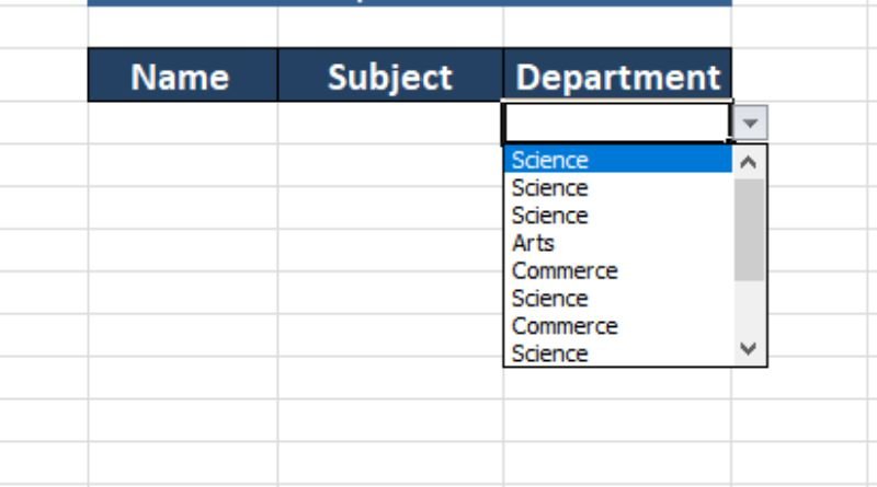
Step 2: Select your field
Once you’ve selected your field, click in the second row of the new column and select the intersection. The cells that display should be updated to show any selections made. This means you can now create a menu with two columns, one for items and one for selections. Select your first item in the Item column and make sure to select Show Text as List from the Styles section. In the selections column, enter either a number or letters to correspond to each item.
Step 3: Modify your drop-down list
It’s also important to make sure the items in your list don’t contain any other symbols, such as asterisks or slashes. Finally, enter the range that includes all the items you want to show in your drop-down list. For example, if you are using column A and want the user to be able to select a letter, use cells A1:A26. If you’re looking for more information on how to create a simple drop-down list, visit our blog post on How to Create an Excel Drop Down List.
Step 4: Add additional columns if necessary
. Finally, choose where you want your list to appear in your worksheet. Go back to the Data tab and double-click in any cell where you want the first item in your drop-down list to appear. A text box will appear around that cell and a cursor will show up on it, ready for typing. Choose List Values from the Sort & Filter group on the Data tab. Select Comma Separated Value (CSV) if prompted and click OK. In this dialog box, specify which column contains your data by highlighting one of them and clicking Add or Change Columns.