Why You Should Use an Excel Drop Down List from Another Tab

If you’re using Excel to create lists, you may be using the AutoFilter drop down menu to make it easier to find the information you’re looking for. However, if you have several lists of similar data within the same spreadsheet, an Excel drop down list from another tab makes it easier to distinguish between each list and gives your spreadsheet an overall cleaner look and feel. Follow these steps to learn how to create an Excel drop down list from another tab in three easy steps!

What are they?

You can save a ton of time if you make your drop down list in another tab and bring it into the tab you’re working on with a simple cut and paste. That way, when you have to edit the list or add items to it, all you have to do is update the source file. You don’t have to continually go back and forth between tabs. Plus, there’s less clutter so it’s easier to find what you’re looking for when there are multiple tabs open. Once you create the drop down list in one tab, just copy and paste it into the other tabs where you need them. Then rename each tab as needed to match your needs (e.g., Pizza, Chinese Food, etc.). Now whenever you need a new item added, just open up that specific tab and edit away!

When should you use them?

Excel drop down lists are a powerful tool for managing your data. It can save you time, make your spreadsheet look more professional, and allow you to access various data sets without having to switch tabs on your workbook. We recommend using these whenever possible, so that each of the data sets stay organized and distinct from one another. When creating this list, you should select cell A1 as the location of the list, which will be copied down in rows. After typing in this information into cell A1, type in =data set followed by a comma and then by B2:B100 or whatever number corresponds with your desired row number. Finally, type & followed by a space before copying over the next column’s heading text with paste special (copy).

Step-by-step instructions

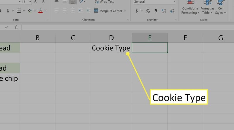
1. In your spreadsheet, select the field you want to display in a drop down list.
2. Select Data, Validation Rules and set the option Input Message: Enter a message (or none) that will be displayed when the data validation fails. In this case, enter ‘Choose a country’.
3.  Click on the Data tab again and select Data Validation from the Tools menu.
4.  Choose List with Values From Another Sheet
5.  Make sure Use Relative References is checked
6.  Click on the arrow beside Source and choose MyTableSheet!Country
7.  Choose OK
8.  When prompted for a location for another sheet or workbook
9.  type or browse to MyTableSheet!A10 10.